Here is a computational problem given to me by Vinayak Vatsal. Given the Riemann theta function
and related Riemann theta function with characteristic
compute for and various with . The definitions of the matrices are
Below are some computations done in an iPython notebook using abelfunctions. You can download the notebook itself here, which requires that abelfunctions be installed in order to execute.
In [1]:
import numpy
import matplotlib
import matplotlib.pyplot as plt
from mpl_toolkits.axes_grid1 import ImageGrid
import matplotlib.colors

from abelfunctions import RiemannTheta
In [2]:
A = numpy.matrix(
    [[2, 1, 1],
     [1, 4, 1],
     [1, 1, 6]],
    dtype = numpy.complex)
B = numpy.matrix(
    [[23, -5, -3],
     [-5, 11, -1],
     [-3, -1, 7]],
    dtype = numpy.complex)
In [3]:
# construct the funciton we want to compute the values of:
#
# theta[sigma,0](0,zM)
#
# where sigma, z, and M can vary

def vitsal(z, sigma, mat):
    # construct the Riemann (period) matrix tau and 2tau
    tau = z*mat
    tau2 = 2*tau

    # compute theta with characteristic (RiemannTheta.characteristic()
    # is untested.)
    dot = numpy.dot(sigma.T, numpy.dot(tau2, sigma))
    scale = numpy.exp(2*numpy.pi*1.0j * dot).item()
    arg = numpy.dot(tau2, sigma)
    return scale * RiemannTheta(arg, tau2)

# vectorize over z since we want to see the behavior of
# this function for some varying z
vitsal = numpy.vectorize(vitsal, excluded=['sigma', 'mat'])We (arbitrarily) choose and . Although, the plots in the following section suggests that the choice of in the upper half plane doesn’t matter except, possibly, in convergence rate of the implementation of the Riemann theta function to the suggested value of the function. That is, it seems like the truncated sum of the Riemann theta function converges to the actual value as we add more terms faster for large.
In [4]:
def print_values(z, mat):
    # constuct list of all half integer characteristics
    halfs = [0,0.5]
    sigmas = []
    for s1 in halfs:
        for s2 in halfs:
            for s3 in halfs:
                sigmas.append(numpy.matrix([s1,s2,s3]).T)

    # for each characteristic, print characteristic and
    # value of theta function
    for sigma in sigmas:
        val = vitsal(z, sigma=sigma, mat=mat)
        print 'sigma.T: %s\tvalue: %s'%(sigma.T, val)
In [5]:
print_values(1.0j, A)Out[5]:
sigma.T: [[0 0 0]]      value: (1.00000697473+0j)
sigma.T: [[ 0.   0.   0.5]]      value: (6.52457377777e-09+0j)
sigma.T: [[ 0.   0.5  0. ]]      value: (6.9877095594e-06+0j)
sigma.T: [[ 0.   0.5  0.5]]      value: (2.2795992109e-14+0j)
sigma.T: [[ 0.5  0.   0. ]]      value: (0.00373488548776+0j)
sigma.T: [[ 0.5  0.   0.5]]      value: (1.21842677994e-11+0j)
sigma.T: [[ 0.5  0.5  0. ]]      value: (1.30369858713e-08+0j)
sigma.T: [[ 0.5  0.5  0.5]]      value: (1.58402415218e-19+0j)
In [6]:
print_values(2.0j, A)Out[6]:
sigma.T: [[0 0 0]]      value: (1.00000000002+0j)
sigma.T: [[ 0.   0.   0.5]]      value: (4.24116597336e-17+0j)
sigma.T: [[ 0.   0.5  0. ]]      value: (1.21615991209e-11+0j)
sigma.T: [[ 0.   0.5  0.5]]      value: (5.15790006267e-28+0j)
sigma.T: [[ 0.5  0.   0. ]]      value: (6.97468471242e-06+0j)
sigma.T: [[ 0.5  0.   0.5]]      value: (1.47903977386e-22+0j)
sigma.T: [[ 0.5  0.5  0. ]]      value: (4.24116597336e-17+0j)
sigma.T: [[ 0.5  0.5  0.5]]      value: (6.27280941128e-39+0j)
In [7]:
print_values(1.0j, B)Out[7]:
sigma.T: [[0 0 0]]      value: (1+0j)
sigma.T: [[ 0.   0.   0.5]]      value: (2.81426845749e-10+0j)
sigma.T: [[ 0.   0.5  0. ]]      value: (9.81431759353e-16+0j)
sigma.T: [[ 0.   0.5  0.5]]      value: (1.47903461596e-22+0j)
sigma.T: [[ 0.5  0.   0. ]]      value: (4.16240046723e-32+0j)
sigma.T: [[ 0.5  0.   0.5]]      value: (1.79873633572e-33+0j)
sigma.T: [[ 0.5  0.5  0. ]]      value: (1.79873633572e-33+0j)
sigma.T: [[ 0.5  0.5  0.5]]      value: (4.16240046723e-32+0j)
In [8]:
print_values(2.0j, B)Out[8]:
sigma.T: [[0 0 0]]      value: (1+0j)
sigma.T: [[ 0.   0.   0.5]]      value: (7.9201069508e-20+0j)
sigma.T: [[ 0.   0.5  0. ]]      value: (9.63208298267e-31+0j)
sigma.T: [[ 0.   0.5  0.5]]      value: (2.18754339521e-44+0j)
sigma.T: [[ 0.5  0.   0. ]]      value: (1.73255776496e-63+0j)
sigma.T: [[ 0.5  0.   0.5]]      value: (3.23545240544e-66+0j)
sigma.T: [[ 0.5  0.5  0. ]]      value: (3.23545240544e-66+0j)
sigma.T: [[ 0.5  0.5  0.5]]      value: (1.73255776496e-63+0j)
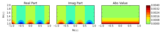
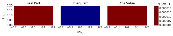
We now draw contour plots for the real, imaginary, and absolute value of the theta function for various in the upper half plane. We chose because it was the only characteristic resulting in a theta value of 1. We chose because it seems to be the one most sensitive to changing and the furthest away from zero for small values of .
In [9]:
# computing the value of the theta function for various z

# set the sigma, z-grid size, and plotting window
sigma = numpy.matrix([0,0,0]).T
N = 64
zre_left, zre_right = -0.2,0.2
zim_left, zim_right = 1,1.2

# compute theta for all of these z
x = numpy.linspace(zre_left, zre_right, N)
y = numpy.linspace(zim_left, zim_right, N)
X,Y = numpy.meshgrid(x,y)
Z = X + 1.0j*Y
V = vitsal(Z, sigma=sigma, mat=A)
In [10]:
# a fancy plotting function so we can see the real, imaginary, and
# absolute values with the same colorbar. took more time to write this
# than the rest of the code in this notebook

def fancy_plot(X, Y, V, figwidth=10):
    # (... omitted for brevity ...)
In [11]:
fancy_plot(X, Y, V)Out[11]:
In [12]:
# same as above, but with sigma = [0.5,0,0]

# set the sigma, z-grid size, and plotting window
sigma = numpy.matrix([0.5,0,0]).T
N = 64
zre_left, zre_right = -1,1
zim_left, zim_right = 1,2

# compute theta for all of these z
x = numpy.linspace(zre_left, zre_right, N)
y = numpy.linspace(zim_left, zim_right, N)
X,Y = numpy.meshgrid(x,y)
Z = X + 1.0j*Y
V = vitsal(Z, sigma=sigma, mat=A)

# plot
fancy_plot(X, Y, V)
Out[12]: