Learning Reinforcement Learning - Part 1

This is the first of a series of posts where I teach myself reinforcement learning. I want these posts to be somewhat exploratory in that I’ll be learning about the topic along the way and sharing the questions that I would ask myself when learning something for the first time. As a result, they may not be as clear as some of the well-written introductory reinforcement learning essays out there. I hope it will still be useful to someone even if my explanation at any given point in time is incomplete. But hey, that’s science, baby.

My trip down reinforcement lane is motivated in part by the usual “self-development for long term career growth blah blah” but, in reality, I want to make a Blood Bowl bot.

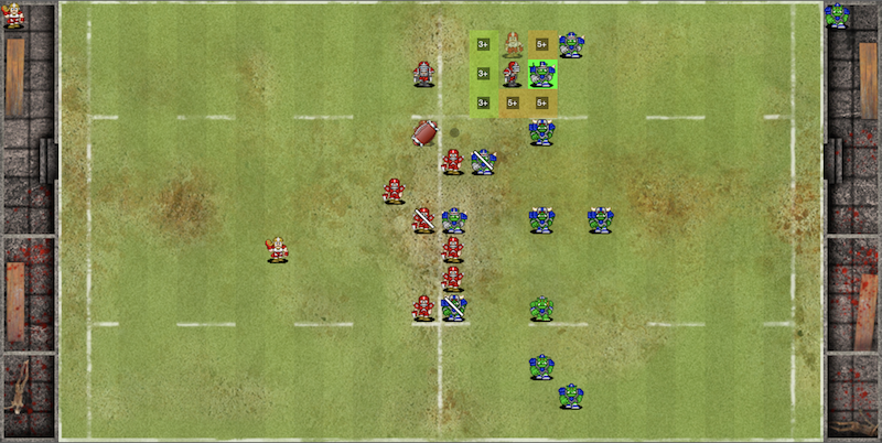
Blood Bowl is a turn-based fantasy football strategy game played on a $26 \times 15$ grid. Two coaches field eleven players each and the object of the game is to score more touchdowns than the opponent. During your turn you can direct players to perform actions like moving, passing, blocking, and fouling. In order to successuflly perform certain actions you need to roll one or two six-sided dice and get a sufficiently high result. Failing any action with any player results in a turnover where it immediately becomes the opponent coach’s turn.

A typical mid-game state. Example shown using the FUMBBL game cilent.

I have been playing Blood Bowl off and on ever since I started college and am recently involved in a league with some friends. It’s a great strategy game about managing risk with a really fun theme. However, Blood Bowl is a terrible place to begin in my reinforcement learning quest because it is a very complicated game. Before fighting dragons I will fight goblins and, instead, I will begin with a classic toy problem called the cart-pole problem.

The cart-pole problem consists of a cart which can move left and right along a track and a pole attached to the center of the cart. The object of the game is to keep the pole upright as long as possible by only moving the cart left and right. For each time step where the pole remains standing we get a point. We lose the game if either the pole leans over more than fifteen degrees or if the cart moves too far away from the center.

Much easier than Blood Bowl.

The Game of Reinforcement Learning

The object of reinforcement learning is to train an agent to interact with an environment in some optimal way. This is done making observations on the current state of the environment, determining an action in response to that observation, and receiving a resulting reward for taking that action. The goal is to determine which set of actions will produce the most reward. Specifically, at each time step $t$ we observe a state $s_t \in \mathcal{S}$ from an environment, execute an action $a_t \in \mathcal{A}$ in response within that environment, and receive a reward $r_t \in \mathcal{R}$. At each time step we wish to maximize the cumulative future reward $R_t = \sum_{s=t}^T \gamma^{s-t}r_s$ where $\gamma \in (0,1)$ is a discount factor and $T$ is the time-step at which the simulation, also referred to as an episode, ends. Note that the cumulative future reward is a prediction of how well the agent will perfom in the future; maximizing this value is similar to determining an optmial behavior policy.

In the cart-pole example the agent is the mechanism which decides how to move the cart. At each time step the agent can move the cart either one unit to the left or one to the right. The state is the tuple $s_t = (x_t, dx_t, \phi_t, d\phi_t)$ of cart position and velocity as well a pole angle and angular velocity. The corresponding reward is equal to one if the pole remains standing and zero otherwise. In Blood Bowl the state includes positional information like player-occupied spaces, player tackle zones, and ball location as well as non-positional information like the current weather, if we are the kicking or receiving team, and the current score. The action space includes moving a player to a given location, electing to tackle an opponent, and passing the ball to a teammate. The reward function can be as simple as setting $r_T = 1$ for winning a game or we can include additional rewards for mid-game results such as scoring a touchdown, knocking out an opponent, or causing a fumble.

Assume we’re given some behavior policy $\pi = \mathbb{P}(a | s)$ that determines which actions are likely to maximize reward from a given state. In the cart-pole problem we can use $\pi_\text{random}$ where we pick a random direction no matter the step. A likely better alternative is the policy $\pi_\text{natural}$ where we move the cart left if the pole is leaning to the left and vice versa. I call this the “natural” policy because when I try to balance a pen on my hand my instinct is to follow the pen with my hand. One way to evaluate policy performance given a state-action pair is by using an action-value function,

$Q_\pi(s,a) = \mathbb{E}\left[R_t \big| s_t=s, a_t=a, \pi \right].$

That is, the action-value function returns the expected cumulative future reward for carrying out an action $a$ on a state $s$ based on the policy $\pi$. However, we don’t know if our perscibed policy is an optimal one. Therefore, we assume that there exists some optimal action-value function,

$Q^*(s,a) = \max_\pi Q_\pi(s,a),$

and we wish to find the policy $\pi$ at which the maximum is achieved, if it exists.

Deep Reinforcement Learning

In deep reinforcement learning our we start with a parmeterized action-value function, $Q(s,a; \theta)$, and wish to learn the values of the parameters $\theta$ such that,

$Q(s,a;\theta) \approx Q^*(s,a).$

Our model for the action-value function can be simple: perhaps we’re trying to find a best-fit line/hyperplane through the action-state space. The “deep” part of deep reinforcement learning is to let $Q(s,a;\theta)$ be a deep neural network and learn the optimal parameters $\theta$ based on observation, or in our case, repeated simulation of the environment. But in order to train a neural network to approximate a function we need to minimize a loss function. Over the past few years a number of loss functions have been proposed and I will look into them over time. But many of them seem to begin with the fact that the action-value function obeys the Bellman equation: let $s$, $a$, and $r$ be the current state, action, and corresponding return. Let $s'$ be the next state. Then,

$Q^*(s,a) = \mathbb{E}_{s' \in \mathcal{S}} \left[ r + \gamma \max_{a'} Q^*(s',a') \big| s, a \right].$

From this we construct the loss function,

$L(\theta_i) = \mathbb{E}_{s \in \mathcal{S}, a \in \mathcal{A}} \left[ \left(y_i - Q(s,a; \theta_i) \right)^2 \right],$

where,

$y_i = \mathbb{E}_{s' \in \mathcal{S}} \left[ r + \gamma \max_{a'}Q(s', a'; \theta_{i-1}) \right].$

What I find interesting about this formulation is that the learned policy is implicit. That is, the model is directly predicting the action-value function. The learned policy, I suppose, would be the action $a^*$ that produces the largest action-value $Q(s, a^*)$ for a given state $s$. That is,

$\pi(s) = \mathbb{P}(a | s) = \text{argmax}_a Q(s, a; \theta).$

Algorithm: Deep Q-Network

The most basic algorithm I could find for this deep learning approach is in [Minh. et al. 2013]. Because deep learning methods need to draw batches of data to learn from the algorithm introduces replay memory: a fixed-length buffer for storing previous state-action-reward-next state tuples. The replay memory mechanism is simple in that batches are sampled uniformly from from the past $N$ tuples and that no particular tuples are assigned greter value than others. It probably works fine but it might be a better idea to assign weights to each tuple proportional to reward. Though, that might lead to poor local mimnima if not enough exploration is allowed.

Algorithm (Basic Deep Q-Learning) Let $\mathcal{D} = \{ (s_j, a_j, r_j, s_{j+1})\}$ contain the replay memory of state, action taken, reward received, and subsequent resulting state from all past episodes. For each episode and for each time step $t$,

1. Select an action:
   1. With probability $\epsilon$ execute a random action, $a_t$. (Exploration)
   2. Otherwise, determine the action, $a_t = \max_a Q^*(s_t, a; \theta)$ with maximal cumulative future reward from the current state of the deep Q-network.
2. Execute and store:
   1. Execute $a_t$ and observe the corresponding reward $r_t$ and next state $s_{t+1}$.
   2. Store $(s_t, a_t, r_t, s_{t+1})$ in $\mathcal{D}$.
3. Learning step:
   1. Sample $(s_j, a_j, r_j, s_{j+1}) \sim \mathcal{D}$.
   2. Set $y_j = r_j,$ if the state $s_{j+1}$ was terminal. Otherwise, $y_j = r_j + \gamma \max_{a'} Q(s_{j+1}, a'; \theta)$.
   3. Perform a gradient descent step on $L(\theta)$.

To summarize we use the model, which is initialized with random parameters and therefore makes random decision, to act upon the environment storing the results into memory. During training we perform gradient descent on the model’s predicted action-value scores compared to the actual observed reward.

In my next post I will begin implementing this algorithm using MXNet; as an AWS employee I am of course legally obligated to use the deep learning framework blessed by my employer. (The real reason: I made some contributions a while back so it’s the framework I’m most familiar with.) Instead, I will be using Pytorch. According to some people this particular deep learning framework is seeing the most use and usage growth in research. For my own benefit, as well as curiosity in how Pytorch does things, I will follow the invisible hand of the market.