Learning Reinforcement Learning - Part 2

In my previous post I described how reinforcement learning can be represented as approximating an optimal action-value function $Q(s, a)$ that assigns a reward to a given state-action pair. The deep learning approach is to learn this function using a model $Q(s, a; \theta) \approx Q^*(s, a)$. In this post I will implement the following Q-learning algorithms and measure their performance on the cart-pole problem:

• Deep Q-Learning [Minh et. al. 2014]
• Double Deep Q-Learning [van Hasselt et. al. 2016]
• Dueling Q-Learning [Wang et. al. 2015]

You can find all of my code in this GitHub repository. This link is to the state of the repository at the time of this post.

Main Loop and Architecture

The high-level, per-episode main loop is as you might expect. While the environment is in a non-terimal state we (1) read the current state, (2) decide on an action using the current state of our agent model, and (3) step the environment forward based on our action. Additionally, we (4) remember the relevant input-output training information and (5) run a single update step on the model, minimizing the loss defined above.

def run_episode(agent, environment, max_iterations=500, ...):
    environment.reset()
    is_terminal = False
    num_iterations = 0
    total_reward = 0

    while (not is_terminal) and (num_iteratios < max_iterations):
        state = environment.state
        action = agent.act(environment)
        next_state, reward, is_terminal, _ = environment.step(action)
        
        agent.remember(state, action, reward, next_state, is_terimal)
        agent.update()
        
        total_reward += reward
        num_iterations += 1
        
    return total_reward

From here the main difference between the algorithms we will be testing is the implementation of agent.update(). See the code for the details, but I decided to create two separate Agent and Model objects where each Agent contains a Model. The Agent is a problem-specific construction that defines how to act upon and remember a given environment. The Model defines the update step and stores the underlying neural network. That is, the Agent acts as a “translator” between the environment and the model. With this structure I can more easily test different models (deep Q, double Q, dueling Q) on the same problem.

Deep Q-Learning

The basic deep Q-learning algorithm described in [Minh et. al. 2014] is the same as the one I shared in the previous post. Using some propoerties of Q-functions, the learning process on the network parameters is defined by minimizing the L2-loss between $Q(s, a; \theta_t)$,

$L(\theta_t) = \left( y_t - Q(s_t, a_t; \theta_t) \right)^2,$

where the target value $y_t$ is given by,

$y_t = r_t + \gamma \max_{a'} Q(s_{t+1}, a'; \theta_t).$

The update step acts on a batch of state, action, reward, next state, and terminal flag tuples. In the below code snippet, self.net is the underlying neural network approximation $Q(s, a; \theta) \approx Q^*(s, a)$, where $\theta$ represents all of the neural network parameters. In the cart-pole problem I chose a three-layer linear network with thirty-two hidden layers and ReLU activations.

class DeepQModel(Model):

   def update(self, states, actions, rewards, next_states, are_terminal):
        self.net.train()
        batch_size = len(states)

        # compute the q-values from the current states corresponding to the
        # given actions
        current_qvalues = self.net(states).gather(1, actions)

        # compute target q-values from next states corresponding to the
        # maximally beneficial actions
        next_qvalues = self.net(next_states).max(1, keepdim=True)[0]
        expected_qvalues = rewards + (1-are_terminal)*self.discount_factor*next_qvalues

        loss = self.loss_function(current_qvalues, expected_qvalues.detach())
        self.optimizer.zero_grad()
        loss.backward()
        self.optimizer.step()
        return current_qvalues

Note that we call detach() on the expected/target Q-values, $y_i$, because we only perform gradient descent on $Q$ evaluated on the current state-action pair.

Double Deep Q-Learning

Unfortunately, as we will see in the “Measurement” section below, the learning process is still appears unstable; the average per-episode reward climbs to local maximum before dropping significantly and (maybe) slowly climbing back up. This may be due to the choice of learning rate and, therefore, the neural network itself jumping to other local minima. However, it was observed in [van Hasselt et. al.] that the deep Q-learning method has a tendency to over-estimate action values. More importantly, the authors show that this over-esimation results in an upward bias of the predicted action-value function.

The paper proposes a solution to this action-value over-estimation problem called “double deep Q-learning”. In “standard” deep Q-learning the target value is given by,

$y^{DQN}_t = r_t + \gamma \max_{a'} Q(s_{t+1}, a'; \theta_t).$

The over-estimation, in part, comes from using the same network parameters $\theta_t$ to perform both action selection and evaluation. (The action is implicitly selected as the one maximizing the learned action-value function.) Double deep Q-learning separates the two roles by maintaining two sets of network parameters: a set of online parameters $\theta_t$ for action selection and a more conservative set of target parameters $\theta_t'$. The target value then becomes,

$y^{DDQN}_t = r_t + \gamma Q(s_{t+1}, a'; \theta_t'),$

where

$a' = \text{argmax}_a Q(s_{t+1}, a; \theta_t).$

In the original paper, “the update to the target network stays unchanged from DQN, and remains a periodic copy of the online network”. The periodicity depends on the problem but when applied to the Atari 2600 domain the authors updated the target network every ten thousand training steps. However, in other papers I have seen this update step written as the linear interpolation,

$\theta' = \tau \theta + (1 - \tau) \theta', \quad \tau = 0.05.$

I decided to use the linear interpolation approach since that seems to be the standard nowadays. Additionally, this update mechanism is somewhat normalized across application domains: ten thousand steps may be appropriate for Atari because the network is so large and total parameter deltas are large but one hundred might be appropriate for cart-pole. The linear interpolation approach “smoothes out” the potentially rapid changes in the online model. Finally, because of the success of double Q-learning I have noticed in various papers and articles that this is sometimes referred to as deep Q-learning; in other words, the original technique should include a separate target network.

We maintain separate self.target_net model which is used only in the update step:

class DoubleQModel(Model):

    def update(self, states, actions, rewards, next_states, are_terminal):
        self.net.train()
        self.target_net.eval()
        batch_size = len(states)

        # compute current q-values from the current states corresponding to the
        # given actions using the online network
        current_qvalues = self.net(states).gather(1, actions)

        # compute target q-values from next states corresponding to the
        # maximally beneficial actions. Use the online network to determine
        # which action should be taken and the target network to evaluate.
        maximal_actions = self.net(next_states).argmax(1, keepdim=True).detach()
        maximal_qvalues = self.target_net(next_states).gather(1, maximal_actions)
        expected_qvalues = rewards + (1-are_terminal)*self.discount_factor*maximal_qvalues

        loss = self.loss_function(current_qvalues, expected_qvalues.detach())
        self.optimizer.zero_grad()
        loss.backward()
        self.optimizer.step()
        self._update_target_model(0.05)
        return current_qvalues

Again, the online network is used to compute current_qvalues as well as the maximal actions which are fed into the target network.

Dueling Q-Learning

Dueling Q-Learning, described in [Wang et. al. 2015], introduces a method for encoding the value of states rather than state-action pairs. The intuition being that in some problems there exist states where no matter what action you take the environment isn’t affected in any positive way. For example, when the cart-pole is at a sufficiently large angle from the center no amount of fixed velocity movement will correct the pole. In Blood Bowl the chances any actions will turn the game in your favor are significantly reduced when the majority of your team is injured. Therefore, it may be useful to train the network to explicity avoid these low-value states.

We define the value function as the average state-action value across all possible actions under the current policy/network state,

$V_\pi(s) = \mathbb{E}_{a \sim \pi(s)}\left[ Q_\pi (s, a) \right].$

We see that, assuming $Q_\pi \approx Q^*$, a small value of $V$ implies that none or few actions produce a large state-action value. In fact, from this definition it follows that the optimal value function $V^*$ is the one associated with the optimal state-action value function $Q^*$,

$V^*(s) = \max_a Q^*(s,a).$

The paper also defines the advantage function which produces the relative value of each action,

$A_\pi(s,a) = Q_\pi(s,a) - V_\pi(s).$

By definition, the advantage function has mean zero across all actions. Given a state its output is positive for actions that “improve” our situation and negative for detremental actions.

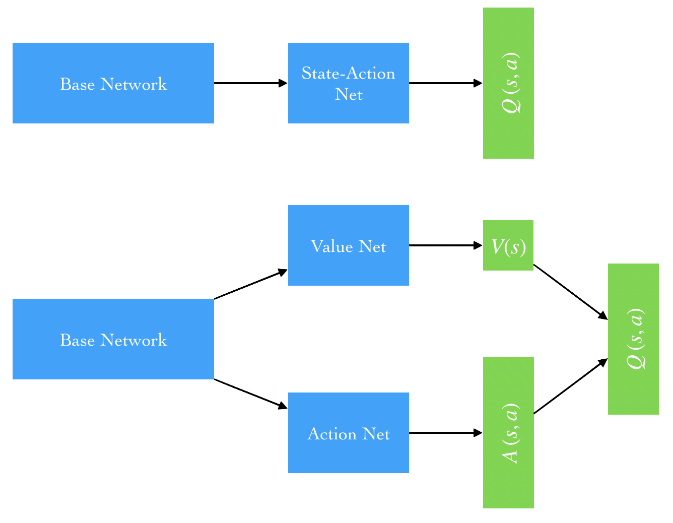
As stated in the paper introduction the goal is to use the value function and advantage function in such a way that we can create a drop-in replacement for other deep Q-learning models. So it is tempting to define $Q_\text{dueling}(s,a) = A(s,a) + V(s)$. However, the authors argue that this formulation suffers from lack of identifiability in that we can achieve the same state-action value for a continum of value function and advantage function values: shift $A$ and $V$ by the same constant. Their solution is to define $Q$ in such a way that the advantage function is forced to have zero advantage,

$Q_\text{dueling}(s,a) = V(s) + A(s,a) - \max_{a'} A(s,a').$

However, the authors found via experimentation that, although the following forumulation loses a bit of the meaning behind the two dueling functions, the learning becomes more stable,

$Q_\text{dueling}(s,a) = V(s) + A(s,a) - \frac{1}{\left| \mathcal{A} \right|} \sum_{a' \in \mathcal{A}} A(s,a').$

(This seems to be a solid example of deep learning as both a science and an art.) With this forumulation we see that the only difference is the Q-value model architecture. That is, we can use either the deep Q-learning or double Q-learning update algorithms as long as we change the model to fit this architecture. Instead of outputting a $\left| \mathcal{A} \right|$-dimensional vector in our network we output $V$ and $A$ and compute the above expression.

Difference between the base network (top) and the dueling network (bottom) for computing the action-value function $Q(s,a)$.

Thankfully, our favorite deep learning framework will handle the gradients for us. Below is the dueling Q-network as custom Pytorch model. Note that we use the same theiry-two layer network as the base but instead send the output to distinct value and advantage functions. We use the double Q-learning algorithm for updates in our experiments.

class DuelingQNet(nn.Module):

    def __init__(self, state_dim, action_dim, **kwds):
        super(DuelingQNet, self).__init__(**kwds)

        self.base_net = nn.Sequential(
            nn.Linear(state_dim, 32),
            nn.ReLU(),
            nn.Linear(32, 32),
            nn.ReLU())

        self.value_net = nn.Linear(32, 1)
        self.advantage_net = nn.Linear(32, action_dim)
        

    def forward(self, x):
        y = self.base_net(x)
        y_value = self.value_net(y)
        y_adv = self.advantage_net(y)
        q_value = y_value + y_adv - y_adv.mean(1, keepdim=True)
        return q_value

Measurement

The primary metric of success is the total reward resulting from each episode. However, the reward metric tends to be noisy, even when averaged across multiple games, due to the sensitivity of action selection with respect to the network weights. I am guessing that this is in part due to the nature of neural networks but my instinct tells me that it is also due to the use of the max operator: if the Q-values are close within a subspace of actions then any small noise in the model can result in frequent action changes.

Therefore we measure the average reward per epoch of size $T$. In these experimence I chose $T = 1000$; that is, we total the rewards across one-thousand iterations and take the average. The reward function for cart-pole is simple: $r_t = 1$ if the episode is in a non-terimal state. Because the episode maxes out at five-hundred interations a well-trained model will max out at a mean reward of,

$\max \frac{1}{T} \sum_{t=t_i}^{t_i + T} r_t = \frac{2 \times 499}{1000} = 0.998.$

Below is a plot of the mean reward for the three tested algorithms.

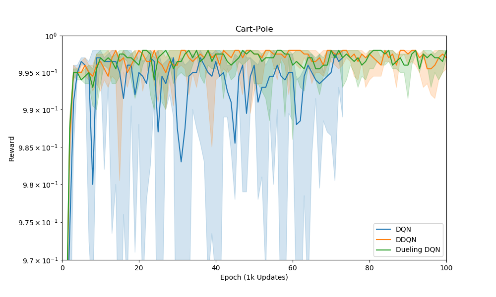
Mean reward per epoch. The shaded regions represent the 10th to 90th percentile range across several experiments. We train for one-thousand episodes so resulting number of epochs depends on the performance of the Q-learning technique.

The original deep Q-learning method is very unstable. In the eyeball-norm the double Q and dueling Q-learning models perform similarly though it does seem that the variance is smaller in the dueling model. Perhaps with a more complex problem the differences between the two methods will come out.

It is also common to track the action-value function, itself, during training. We track the action-values similarly to the way [Minh et. al.] and [van Hasselt et. al.] do in their respective papers: compute the maximum predicted action-value on a set of hold-out states. The action-values are averaged within each epoch consisting of a specified number of minibatch updates. That is,

$\bar{Q}_i = \frac{1}{T} \sum_{t=t_i}^{t_i + T} \max_a Q(s_t, a; \theta_t),$

where $T$ is the size of each epoch. Below is a plot of these average Q-values.

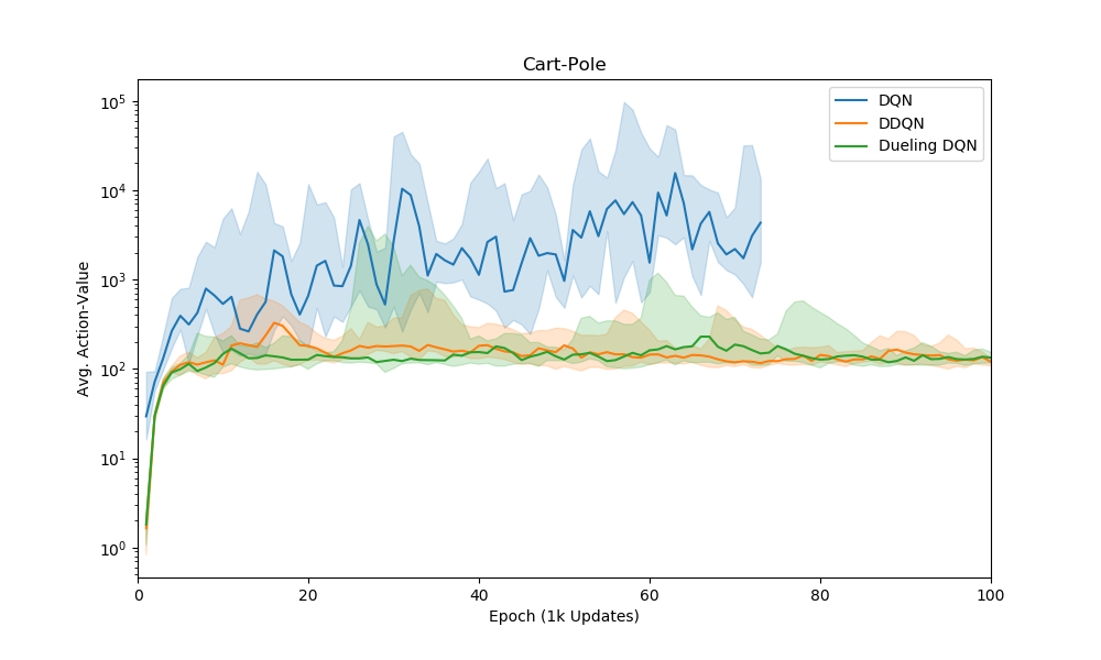
Mean Q-value per epoch. Again, we train for one-thousand episodes so resulting number of epochs depends on the performance of the Q-learning technique.

As discussed in the van Hasselt paper the double Q algorithm is much more conservative in its Q-value estimates. There doesn’t seem to be a difference between that and the dueling Q-network but, again, this may be due to the lack of complexity in the problem. With only two possible actions the averaging procedure in the dueling Q-function definition doesn’t add much difference. Interesting to note, the wild fluctuations and sudden drops in Q-value estimate seem to correspond to the drops in average reward. This is especially clear in the vanilla deep Q-learning method.

Next Time

I now feel like I have a basic understanding of deep Q-learning methods and am ready to apply this to Blood Bowl. However, the first step to doing so is to explore the blood bowl environment a bit and decide on network architecture.